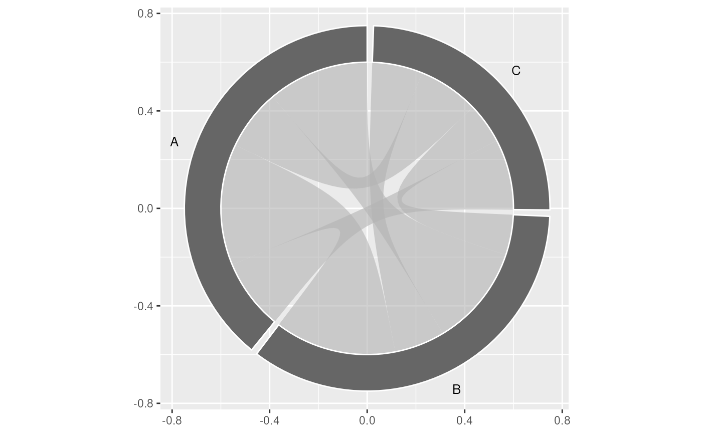
Chord Diagram
geom_chord_diagram.RdChord Diagram
Arguments
- mapping
A
ggplot2::aes()mapping. Must supply at minimumsource,target, andfreq.- data
Data frame. If
NULL, inherits from the plot.- gap_degree
Degrees of gap between sectors (default 2).
- start_degree
Starting angle in degrees for the first sector (default 90).
- direction
1 = counter-clockwise (default), -1 = clockwise.
- inner_radius
Normalised inner radius of the sector ring (default 0.6).
- outer_radius
Normalised outer radius of the sector ring (default 0.75).
- n_bezier
Smoothness: number of points per curve (default 100).
- show_labels
Logical. Draw node labels? Default
TRUE.- arc_params
Named list of additional parameters passed to
geom_chord_arcs.- sector_params
Named list of additional parameters passed to
geom_chord_sectors.- label_params
Named list of additional parameters passed to
geom_chord_labels.
Aesthetics
geom_chord_diagram() understands the following aesthetics
(required in **bold**):
source– name of the originating nodetarget– name of the receiving nodefreq– numeric flow / weightfill– fill colour of ribbons / sectorscolour– border colouralpha– transparency (default 0.6 for ribbons, 1 for sectors)linewidth– border line width